
Central Limit Theorem
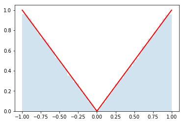
The central limit theorem is a key result in probability theory that helps explain why normal, or Gaussian, distributions are so omnipresent. The setup is that you have distributions for $N$ random variables $x_i$ and you want to know the distribution of $q = \sum_{i=1}^{N} x_i$. Think of each $x_i$ as coming from it's own distribution like in the figure below. For instance, $x_1$ might be the weight of spoons, $x_2$ the weight of forks, $x_3$ the weight of bowls, ..., and $x_N$ of plates in your kitchen. Then $q$ would represent the total weight when you have one of each of those objects. The distribution of weights for each object might be weird because you have some mix-and-match set of silverware from your parents, grandparents, IKEA, and the thrift shop. The central limit theorem says that if you have enough objects (i.e. $N$ is large), then $q$ has a normal (Gaussian) distribution.

Moreover, the central limit theorem states that the mean value of $q$ is given by
\begin{equation} \mu_{q} = \sum_{i=1}^{N} \mu_{x_i} \end{equation}and the variance (standard deviation squared) is given by
\begin{equation} \sigma_{q}^{2} = \sum_{i=1}^{N} \sigma^2_{x_i} \end{equation}if you are having problems with the math displaing, click here
The mean probably isn't surprising because $q$ is just a sum and the integral the defines the mean just distributes across each term. Also, the equation for the variance is the same as the propagation of errors formula we use when we add different measurements together. However, that propoagation of errors formula is derived from the Central Limit Theorem, not vice versa.
This is a collaborative project
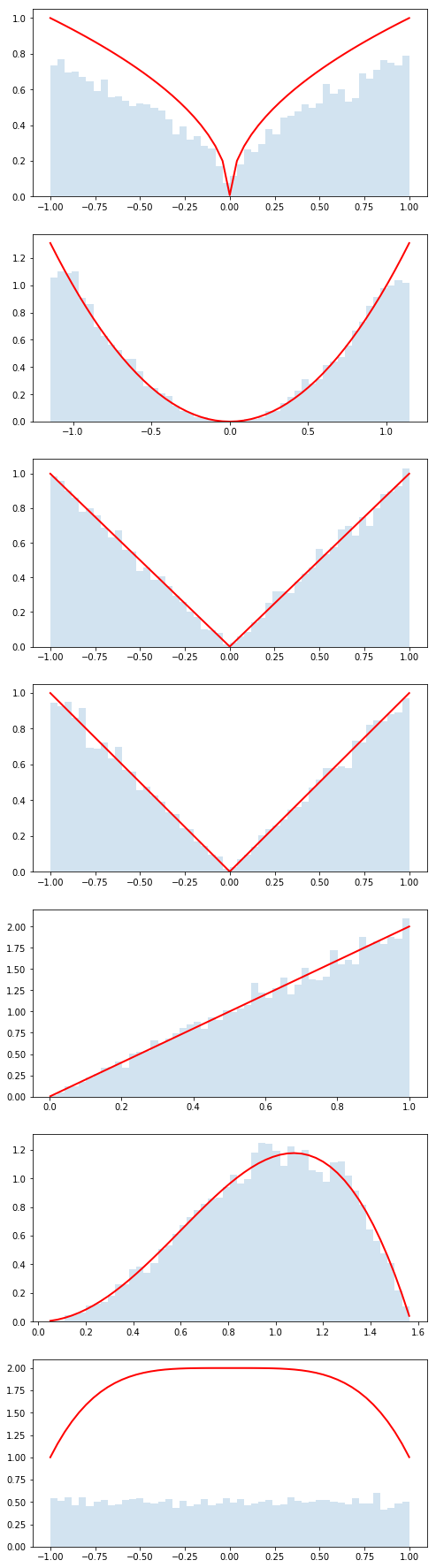
In this repository there is a folder called distributions with several python files. The idea is that each student will create one of these python files and we will use GitHub to collect them. Each of these files has a python class that describes a probability distribution. Each of these classes will define:
x_min, x_max, f_max- used for the accept/reject Monte Carlo sampling algorithmpdf()- the probability density functionmean()- the mean of the pdfstd()- the standard deviation of the pdf
In addition, each of these python classes inherits from BaseDistribution which knows how to run the accept/reject algorithm using the information above (see inside ). In order to generate n_samples from the pdf, you simply call dist.rvs(n_samples), where dist is an instance of one of these python classes.
Naming Convention: Name your file Dist_<netid>.py and your distribution the same way (without the .py). If you want to contribute more than one distribution, you can can add Dist_<netid>_<index>.py, where <index> is 1,2,3,...
Here's an example:
!cat distributions/Dist_kc90.py
%pylab inline --no-import-all
from scipy.stats import norm #will use this for plotting
# import all our distributions
import distributions
# some funny python to make a list of all the distributions for convenience
all_distributions_dict = dict([(name, cls) for name, cls in distributions.__dict__.items() if isinstance(cls, type)])
all_distributions_list = [(cls) for name, cls in distributions.__dict__.items() if isinstance(cls, type)]
# print out their names
all_distributions_dict.keys()
len(all_distributions_dict.keys())
## Do tests
ok_distributions_list=[]
problems=[]
for i, cls in enumerate(all_distributions_list):
    #print(cls)
    try:
        dist = cls()
        N_test = 100000
        #print('will try to generate for %s' %(cls.__name__))
        if dist.pdf(dist.x_min + .3*(dist.x_max-dist.x_min)) < 1E-3:
            print("may have a problem")
            continue

        rvs = dist.rvs(N_test)
        if np.abs(np.mean(rvs) - dist.mean()) > 5*np.std(rvs)/np.sqrt(N_test):
            print("means don't match for %s: %f vs. %f" %(cls.__name__,
                                                          np.mean(rvs), dist.mean()))
            continue

        elif np.abs(np.std(rvs) - dist.std()) > 5*np.std(rvs)/np.sqrt(np.sqrt(1.*N_test)):
            print("std devs. don't match for %s: %f vs. %f" %(cls.__name__,
                                                          np.std(rvs), dist.std()))
            continue
        elif np.abs(np.std(rvs) - dist.std()) / dist.std() > 0.1:
            print("std devs. don't match for %s: %f vs. %f" %(cls.__name__,
                                                          np.std(rvs), dist.std()))
            continue

        elif np.sum(dist.pdf(np.linspace(dist.x_min,dist.x_max,100))<0) > 0:
            print("pdf was negative in some places")
            continue

        else:
            print("%s passes tests, adding it" %(cls.__name__))
            ok_distributions_list.append(cls)
    except:
        print("%s has errors, does't work" %(cls.__name__))
        continue

print("list of ok distributions:",[i.__name__ for i in ok_distributions_list])
problems = [x for x in all_distributions_list if x not in ok_distributions_list]
[i.__name__ for i in problems]
# how many samples for plots?
n_samples = 100000
# Here's an example of usage
dist = distributions.Dist_kc90()
rvs = dist.rvs(n_samples)
counts, bins, edges = plt.hist(rvs, bins=50, normed=True, alpha =0.2)
y = []
for bin in bins:
    y.append(dist.pdf(bin))
plt.plot(bins, y, c='r', lw=2)
dist.std()
fig = plt.figure(figsize=2*plt.figaspect(len(ok_distributions_list)))
for i, cls in enumerate(ok_distributions_list):
    dist = cls()
    rvs = dist.rvs(10000)
    ax = fig.add_subplot(len(ok_distributions_list),1,i+1)
    counts, bins, patches = ax.hist(rvs, bins=50, normed=True, alpha=0.2)
    # depending on how you code up your pdf() function, numpy might not
    # be able to "broadcast" (apply the function for each element of a numpy array)
    # but this should always wrok
    y = []
    for bin in bins:
        y.append(dist.pdf(bin))

    # ok, now plot it
    plt.plot(bins, y, c='r', lw=2)

    # and let's check if the distribution is ok
    print("%s: std from samples = %.2f, std from dist = %.2f" %(cls.__name__,np.std(dist.rvs(n_samples)), dist.std()))
    if np.abs(np.std(dist.rvs(n_samples)) - dist.std()) / dist.std() > 0.1:
        print("looks like a problem with this distribution: ", cls)
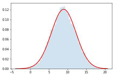
def do_convolution(dist, N):
    n_samples = 10000
    q = np.zeros(n_samples)
    var_q = 0.
    mean_q = 0.

    for i in range(N):
        q = q+dist.rvs(n_samples)
        var_q = var_q + dist.std()**2
        mean_q = mean_q + dist.mean()

    std_q = np.sqrt( var_q )


    counts, bins, patches = plt.hist(q,bins=50, normed=True, alpha=.2)
    plt.plot(bins, norm.pdf(bins,loc=mean_q, scale=std_q), lw=2, c='r')
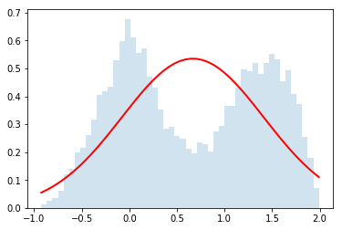
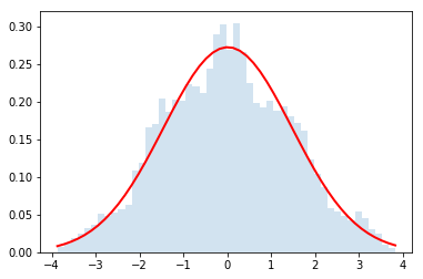
Now let's use it for $N=\{2,4,32\}$
dist = distributions.Dist_kc90()
do_convolution(dist,2)
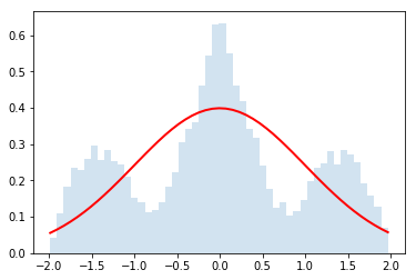
do_convolution(dist,4)
do_convolution(dist,32)
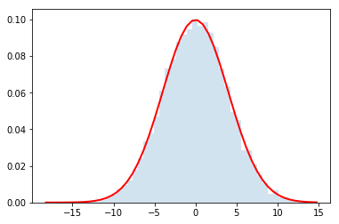
Gorgeous!
np.random.choice(['a','b','c','d'], 10)
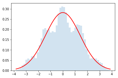
Now let's make a variation on the helper function above
def do_random_convolution(list_of_distributions, N):
    n_samples = 10000
    q = np.zeros(n_samples)
    var_q = 0.
    mean_q = 0.

    for dist_class in np.random.choice(list_of_distributions,N):
        dist = dist_class()
        print(dist_class.__name__, dist.std())
        q = q+dist.rvs(n_samples)
        var_q = var_q + dist.std()**2
        mean_q = mean_q + dist.mean()

    std_q = np.sqrt( var_q )


    counts, bins, patches = plt.hist(q,bins=50, normed=True, alpha=.2)
    plt.plot(bins, norm.pdf(bins,loc=mean_q, scale=std_q), lw=2, c='r')
do_random_convolution(ok_distributions_list,2)
do_random_convolution(ok_distributions_list,4)
do_random_convolution(ok_distributions_list,4)
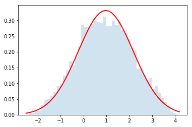
do_random_convolution(ok_distributions_list,32)
Part 2 of project
a) preliminaries
From either master or the branch you used to submit your distribution, update so that you have the current version of cranmer/intro-exp-phys-II.
You can either do this in GitHub desktop by finding the button near the top left or by typing this:
git fetch cranmer master
git merge cranmer/master
Now Create a new branch called "part2"
b) execute the notebook above
c) Make a $\chi^2$ function
Below is a copy of the do_random_convolution function with a new name. Modify it so taht it returns the chi-square quantity that says how closely the observed distribution matches the prediction from the Central Limit theorem.
YOu might want to check out the chi-square-of-distribution notebook
def do_random_convolution_with_chi2(list_of_distributions, N):
    n_samples = 100000
    q = np.zeros(n_samples)
    var_q = 0.
    mean_q = 0.

    for dist_class in np.random.choice(list_of_distributions,N):
        dist = dist_class()
        q = q+dist.rvs(n_samples)
        var_q = var_q + dist.std()**2
        mean_q = mean_q + dist.mean()

    std_q = np.sqrt( var_q )


    counts, bins, patches = plt.hist(q,bins=50, normed=True, alpha=.2)
    plt.plot(bins, norm.pdf(bins,loc=mean_q, scale=std_q), lw=2, c='r')